Step 1. Understand how to use (the ACM) LaTeX template with R Markdown

Note: I’ll assume you’re using RStudio for this tutorial

To use the ACM article template, we’d normally download the latest version from here. For the purposes of this tutorial, however, clone or download this GitHub repo which I set up with just the files you need to follow along and understand how things work. Open the R Project file in the repo’s root folder. Now let’s have a look at the files in the step1 folder:

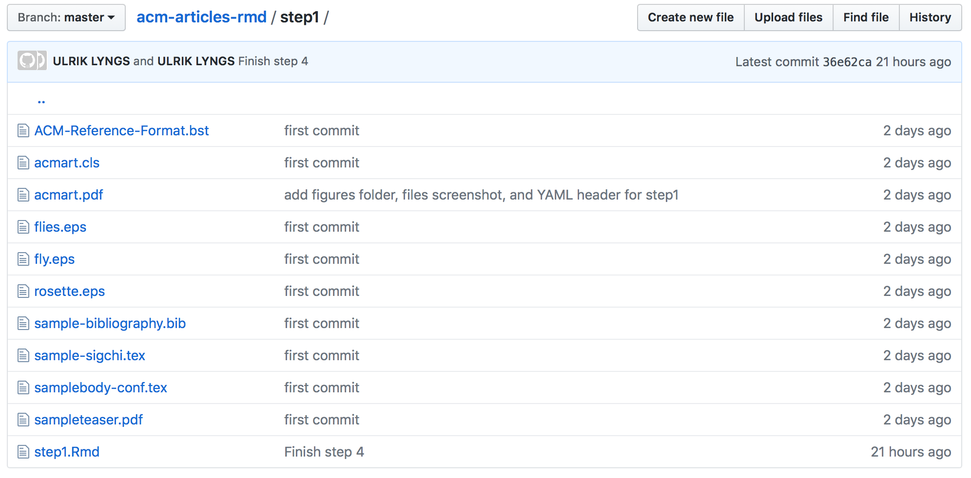
Step 1 files

This folder contains the necessary files to compile the most recent CHI proceedings template (these files are a subset of the files in the acmart-master folder which you can download via the ACM page I linked to above):

• acmart.cls provides the LaTeX class for the new ACM master template
• acmart.pdf provides ACM’s documentation (by Boris Veytsman) for how to use this ACM template
• ACM-Reference-Format.bst provides the bibliography formatting
• sample-sigchi.tex provides the LaTeX template for CHI proceedings (as you can read in the documentation in acmart.pdf, however, you switch the output easily to e.g. CHI Extended Abstracts instead of CHI Proceedings, by changing only the article format argument within this .tex)
• the others are supporting files for the sample content in the template - images (files.eps, fly.eps, rosette.eps, and sampleteaser.pdf), bibliography (sample-bibliography.bib), and sample content (samplebody-conf.tex)

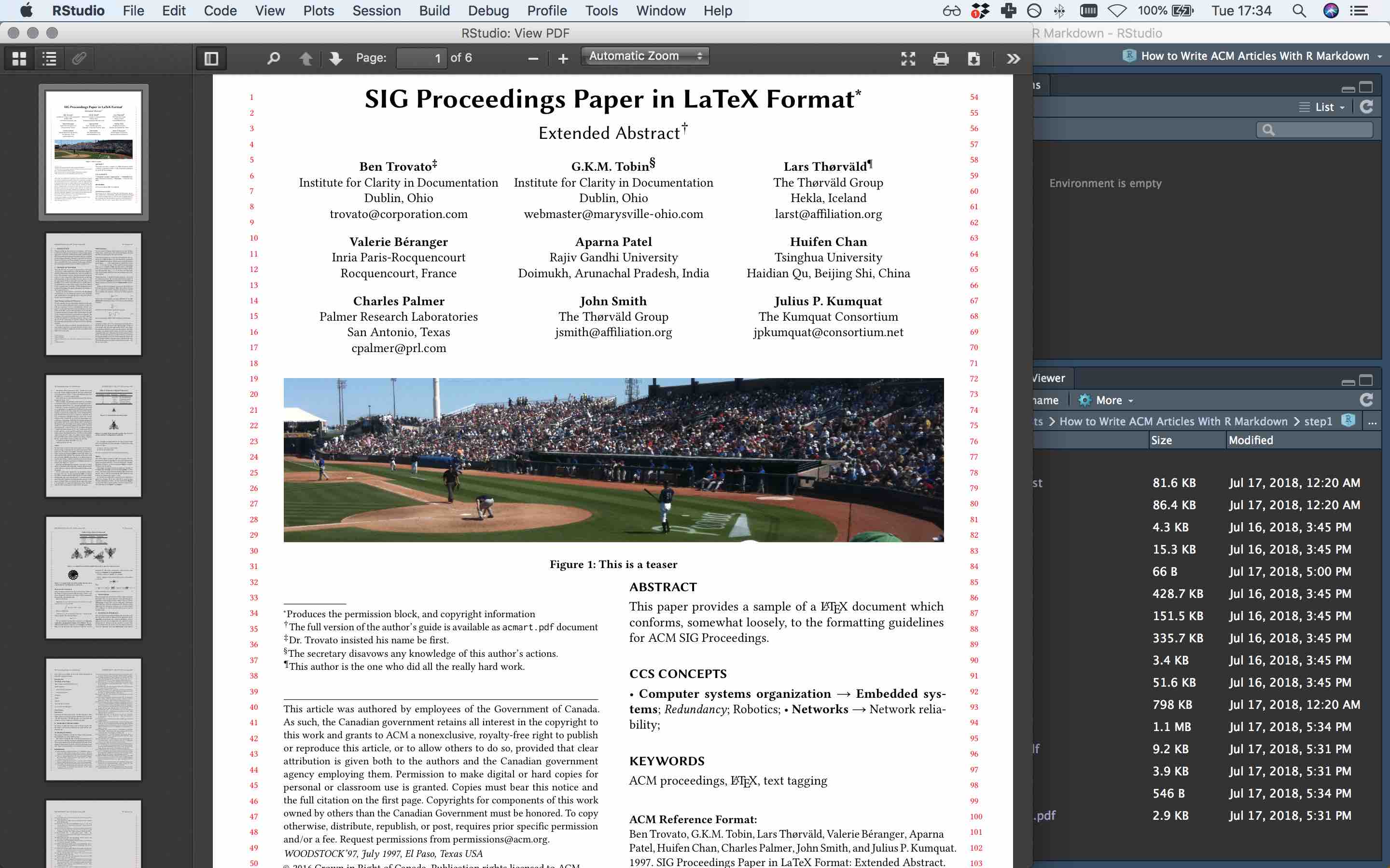
Now, if you open step1.Rmd, you will see that the only thing you need to include in an Rmd file to use an arbitrary LaTeX template (in this case the CHI template) is the following YAML header:

---
output:
    bookdown::pdf_book:
        template: sample-sigchi.tex
---

(Note I use bookdown::pdf_book: as output instead of simply pdf_document. This is because bookdown extends the referencing capability of R Markdown, so that we can reference figures with a syntax that also works when exporting to other formats than LaTeX/PDF.)

If you click ‘Knit’, the CHI proceedings template with sample content should compile to this pdf (if you get an error message, its probably for this reason):

Step 1 compiled to pdf

Step 2. Adjust the LaTeX template to include your content

Ok, so now we know how to compile to an arbitrary template without putting in any content. How do we put in the content from our Rmd file?

To do this, we need to know that pandoc, when compiling from R Markdown to LaTeX, treats content $between dollar signs$ in the LaTeX template as a variable that it should go look for in the Rmd file.

So, for example, if I in sample-sigchi.tex change \title{SIG Proceedings Paper in LaTeX Format} to \title{$title$}, then pandoc will go look for the variable title in the YAML header of the R Markdown file and plug the content of this variable in to the LaTeX template.

So we have a choice: We could go all the way and use variables to put all of the meta data and LaTeX settings for the paper into the YAML header, kinda what I think the ‘rticles’ package intends to do.

I begun doing this myself, but concluded that this is a terrible idea, because we then must keep on top of the detail of all changes that might be made in the future to the ACM LaTeX template to avoid things breaking. What we will do instead, is make minimal changes that just allow us to plug in the body text from the R Markdown document, so that we can reuse the hard work we put in to writing this body text in R Markdown elsewhere. For convenience, we might also want to use variables to plug in the title, abstract, and bibliography file path straight from the Rmd file. If the ACM LaTeX template changes in the future, then we’ll just adjust the latest template with these minimal changes to make it work again.

In other words, I concluded that the route of least effort is to do the following:

1. Plug in paper title from the YAML header (in sample-sigchi.tex change \title{SIG Proceedings Paper in LaTeX Format} to \title{$title$}and in the Rmd file add something like this to the YAML header: title: This is the Greatest and Best Paper in the World (Tribute)

2. Plug in bibliography file from the YAML header (in sample-sigchi.tex, change \bibliography{sample-bibliography} to \bibliography{$bibliography$}. Then add something like bibliography: my-bibliography.bib to the YAML header of your Rmd file.)

3. Plug in abstract from the YAML header file (in sample-sigchi.tex, replace the text between \begin{abstract} and \end{abstract} with $abstract$. Then add something like abstract: This is the greatest and best abstract in the world. Tribute. to your YAML header.)

4. Plug in paper content from the Rmd file body (in sample-sigchi.tex, after \maketitle change \input{samplebody-conf} to $body$. This will make pandoc plug in any content after the YAML header into this section)

All other metadata (author names, whether you need title notes, etc.) we will just set directly in sample-sigchi.tex - it’s not worth the effort (I think) to set up variables for this in your YAML header.

Let’s see what we get when we knit the result (step2/step2.Rmd):

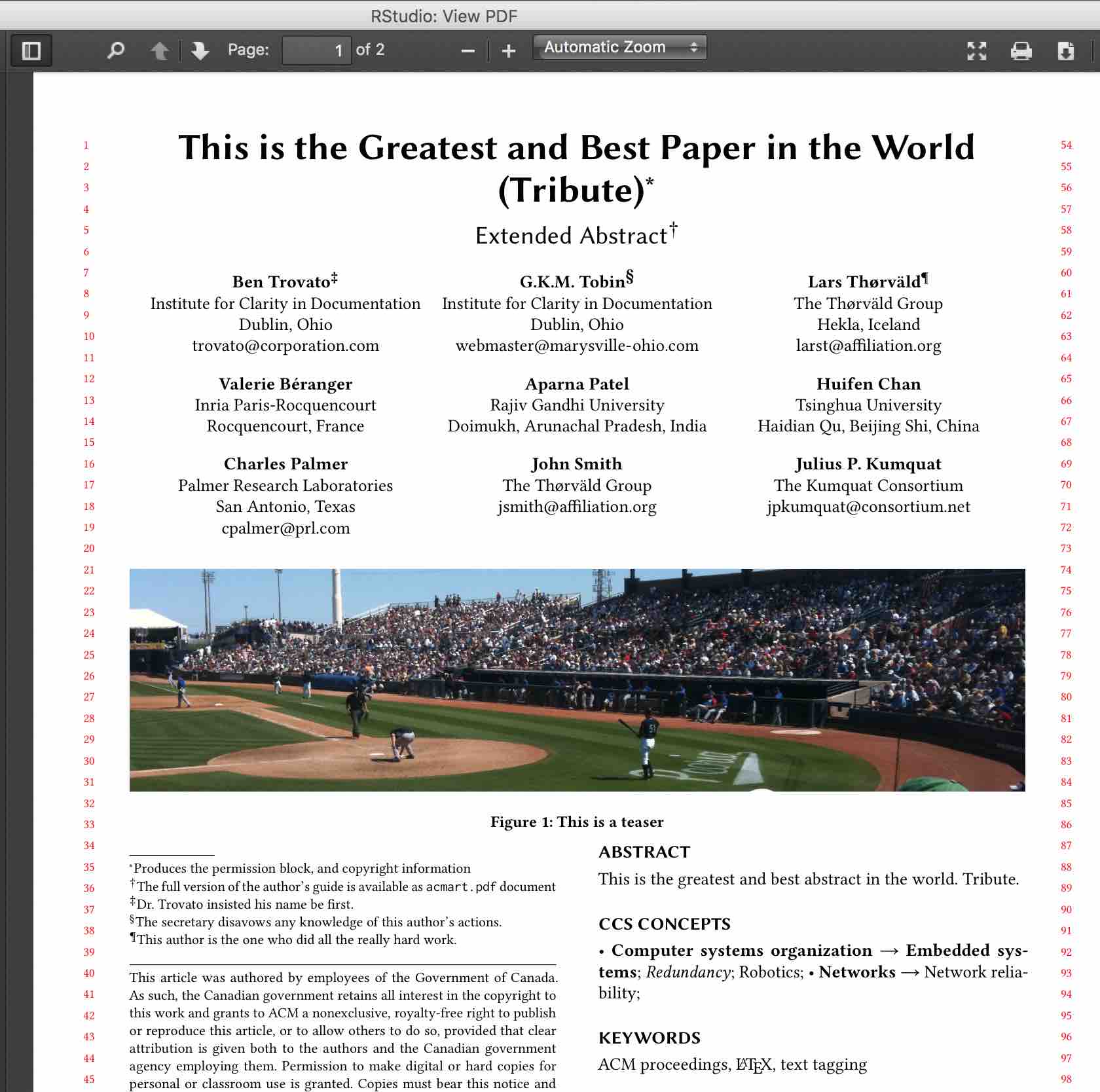
Step 2 compiled first page

Ok, so title and abstract is plugged in correctly from the YAML header. Let’s look at page 2:

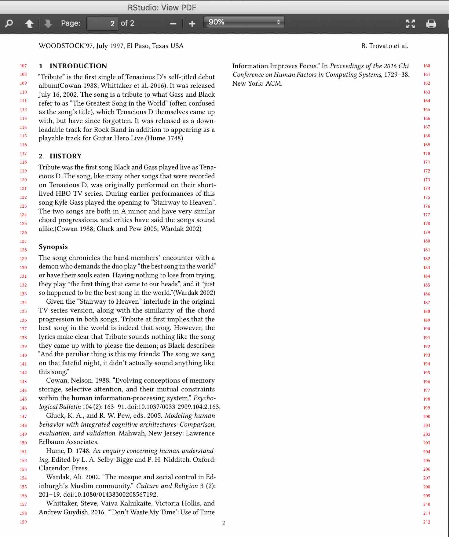
Step 2 compiled second page

Argh! The body content as a whole is input correctly, but the in-text citations are not quite formatted the way we want, nor is the reference list shown in that nice ACM style. What’s going on?

If we add keep_tex: true in the YAML header, as an indented line under bookdown::pdf_document:, we can knit again and inspect the intermediary .tex file that the PDF is generated from. We might notice the following in the .tex file:

(...) playable track for Guitar Hero Live.(Hume 1748)

and in the part containing the references:

\hypertarget{ref-Hume1748}{}
Hume, D. 1748. \emph{An enquiry concerning human understanding}. Edited by L. A. Selby-Bigge and P. H. Nidditch. Oxford: Clarendon Press.

Ahh, now things make sense. In the .tex file, the citations and references have been plugged in as plain text, instead of using the appropriate LaTeX commands. Not quite what we want! Let’s fix this.

Step 3. Make sure citations are shown correctly

Turns out this is easy. Go to the YAML header and under bookdown::pdf_book: add (with indentation) citation_package: natbib. This will make use of the LaTeX natbib package to insert citations into the .tex file, instead of inserting them as plain text. Let’s knit again to see if this made a difference:

Step 3 compiled to pdf

Yup, now it looks right. Let’s have a look at the .tex to see what’s actually going on. Now we see this around the Hume reference:

(...) playable track for Guitar Hero Live.\citep{Hume1748}

So citations are now correctly inserted with \citep{citation-key}, and the bibliography is being generated by LaTeX itself via the final calls to \bibliographystyle{ACM-Reference-Format} and \bibliography{$bibliography$} in sample-sigchi.tex. Success!

Step 4. Handling figures

Let’s get to the fun stuff. We want our plots to be generated straight from R and put automatically into our article, so that we can be awesome and reproducible, right?

First, in our YAML header add fig_caption: true under bookdown::pdf_book. This makes sure our plots are put in a figure environment, and gives us more control over the options of this environment.

Then, in our body text after the ‘History’ paragraph, add the following chunk of R code:

```{r tribute-plot, echo=FALSE, out.width='0.98\\columnwidth', fig.cap="This is a column-width plot of how great Tribute gets over time"}

plot(pressure)

```

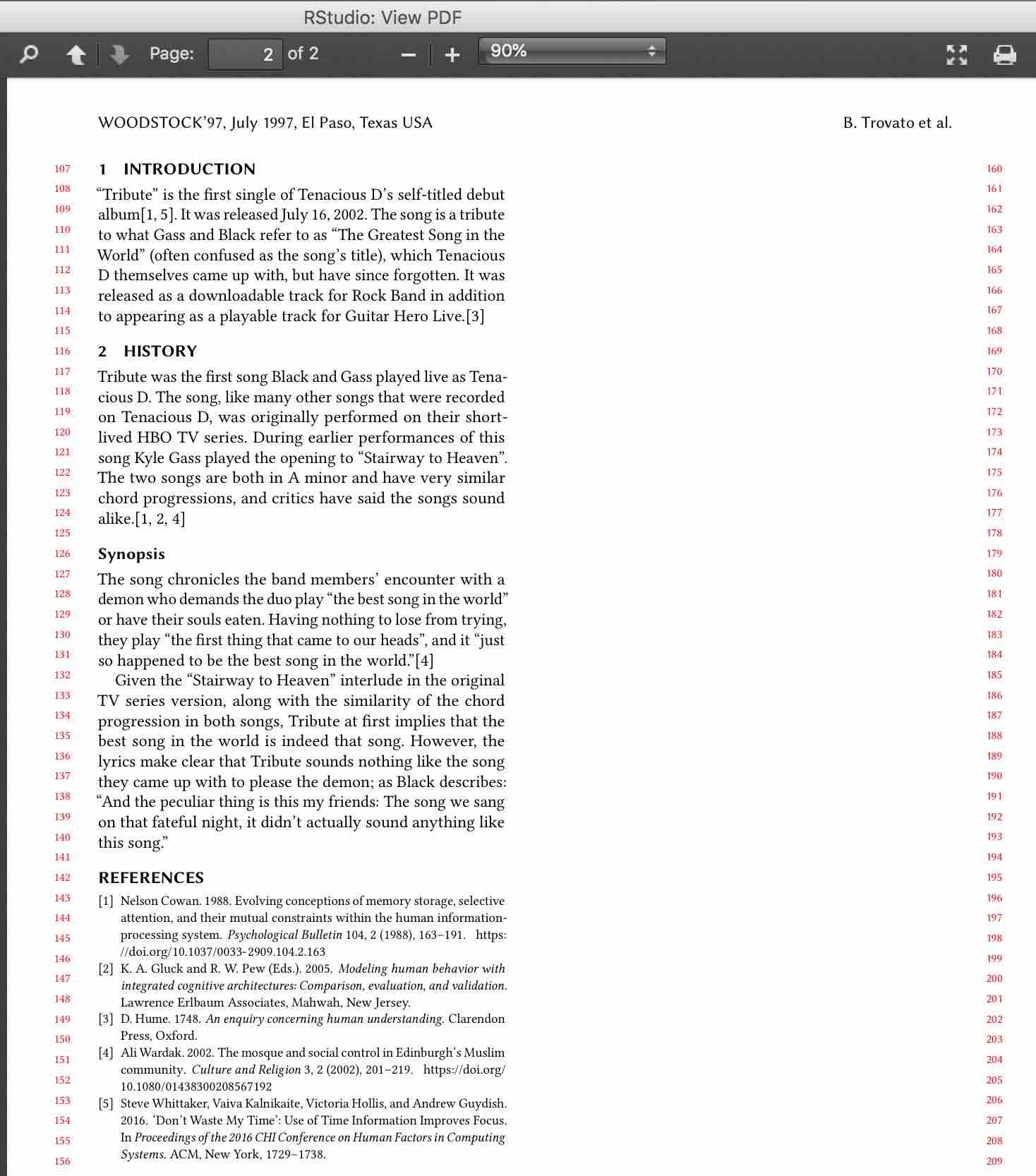
For new initiates, ``` means we want a code chunk, and chunk options are in between { }. r means this chunk contains R code, tribute-plot is the figure label, echo=FALSE says we don’t want to output the code itself, only its output, out.width='0.98\\columnwidth' says we want to restrict the size of the plot to 98% of the width of a column (if you delete this option the plot gets way too big; and note that we must escape the \ with another \), and fig.cap= is followed by a figure caption.

If we knit and inspect the generated .tex file, we can see that this chunk was translated into this corresponding LaTeX:

\begin{figure}
    \includegraphics[width=0.98\columnwidth]{step4_files/figure-latex/tribute-plot-1} 
    \caption{This is a column-width plot of how great Tribute gets over time}
    \label{fig:tribute-plot}
\end{figure}

I.e. R Markdown generates the plot, creates a subfolder and saves the plot as a graphics file in there, then includes this generated file in the .tex file with the LaTeX syntax we’d expect. Magic! (Not to mention a crucial step to automate to avoid errors in the research process!)

The output also looks as we’d expect:

Step 4: figure in column width

Two-column figures

The acm-article template documentation tells us that to include a figure which spans two columns, we should put it in a figure* environment rather than a figure environment. How do we do this? Easy, add fig.env='figure*' to the chunk options:

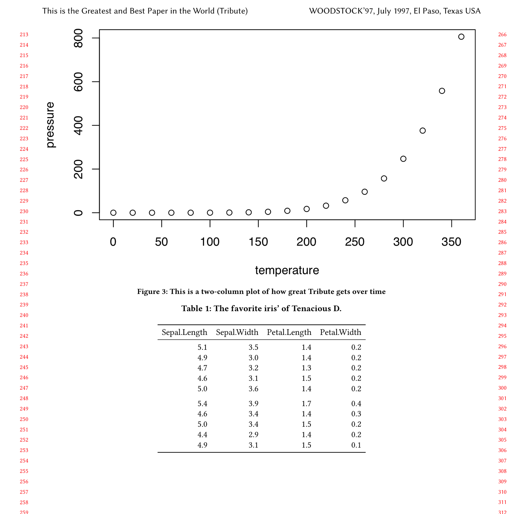
```{r two-col-tribute-plot, fig.env='figure*', echo=FALSE, out.width='0.98\\textwidth', fig.cap="This is a two-column plot of how great Tribute gets over time"}

plot(pressure)

```

(Note also that I changed the output width to out.width='0.98\\textwidth; otherwise the plot width would still be 98% of a column even though it was spanning two columns.)

If we inspect the .tex file, we see this code chunk is translated into this corresponding LaTeX:

\begin{figure*}
    \includegraphics[width=0.98\textwidth]{step4_files/figure-latex/two-col-tribute-plot-1} 
    \caption{This is a two-column plot of how great Tribute gets over time}
    \label{fig:two-col-tribute-plot}
\end{figure*}

And the output looks correct (it’s floating to a new page in our case):

Step 4: figure in full width

Step 5. Handling tables

To automatically grab data from our analyses and create a table in our CHI paper, we’ll use ‘kable’.

For this example, let’s first load the tidyverse package. Let’s add this chunk before the introduction in our Rmd file:

```{r setup, include=FALSE, message=FALSE}
library(tidyverse)
```

(include=FALSE means we don’t want any output from this to be included, and message=FALSE similarly ensures that messages that are shown when a library is loaded are not being interpreted as LaTeX commands. We simply want to load the tidyverse library.)

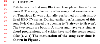
Now, let’s include a subset of the iris dataset as a table in our article. Add this chunk after the Synopsis section:

```{r table-iris, echo=FALSE}
iris %>%
  select(-Species) %>%  #drop the species column
  head(10) %>%          #show just the first 10 rows
  knitr::kable(format = "latex", booktabs = TRUE, caption = "The favorite iris' of Tenacious D.")
```

We pipe the data we want to show into the kable function from the knitr package, and specify that we want the format to be latex, that it should be formatted nicely with booktabs = TRUE, and we also give it a caption.

If we knit and inspect the .tex, we see that the chunk has been translated into this corresponding LaTeX:

\begin{table}
    \caption{\label{tab:table-iris}The favorite iris' of Tenacious D.}
    \centering
    \begin{tabular}[t]{rrrr}
        \toprule
        Sepal.Length & Sepal.Width & Petal.Length & Petal.Width\\
        \midrule
        5.1 & 3.5 & 1.4 & 0.2\\
        4.9 & 3.0 & 1.4 & 0.2\\
        4.7 & 3.2 & 1.3 & 0.2\\
        4.6 & 3.1 & 1.5 & 0.2\\
        5.0 & 3.6 & 1.4 & 0.2\\
        \addlinespace
        5.4 & 3.9 & 1.7 & 0.4\\
        4.6 & 3.4 & 1.4 & 0.3\\
        5.0 & 3.4 & 1.5 & 0.2\\
        4.4 & 2.9 & 1.4 & 0.2\\
        4.9 & 3.1 & 1.5 & 0.1\\
        \bottomrule
    \end{tabular}
\end{table}

And the output looks like this:

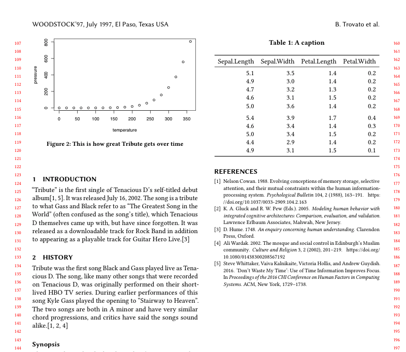
Step 5: table in column width

Awesome! No more errors from whatever obscure means through which you’d otherwise be getting your data into a LaTeX table.

Two-column tables

Finally, the acm-article documentation again tells us that we can get our table to span two columns by putting it in a \table* rather than a \tableenvironment. It turns out that there’s not at the moment any easy way to do this from within R Markdown (the fig.env chunk option doesn’t work with tables when we use the kable function).

Update 7 Aug 2018: Yihui Xie, creator of knitr, told me that this is done just as easily. We simply add table.env='table*' as argument to the kable function:

```{r table-iris-wide, echo=FALSE}
iris %>%
  select(-Species) %>%  #drop the species column
  head(10) %>%          #show just the first 10 rows
  knitr::kable(format = "latex", table.env='table*', booktabs = TRUE, caption = "The favorite iris' of Tenacious D.")
```

Et voilá, our table is put in a \table* environment in the .tex file and now spans two columns:

Step 5: table in full width

Step 6. Referencing our figures and tables

To finish off, how do we reference our figures and tables? Two options - the first is to simply use standard LaTeX syntax (you can use any LaTeX syntax within your Rmd file if you’re compiling it to a PDF). For example:

(...) over time is shown in Figure \ref{fig:col-width-tribute-plot}.

That’s fine, but if you want to keep the option of outputting to another format than PDF in the future, e.g. gitbook or Word, you’ll want to use bookdown’s slightly different syntax:

(...) over time is shown in Figure \@ref(fig:tribute-plot).

Either way, the .tex output is the same, and so is the result:

Step 6: referencing figures and tables

Step 7. Celebrate!

You now know how to use R Markdown alongside the ACM master templates. Yay for reproducible research!